Learn Excel Pivot Table to skill up - Simplest Example

What we Learn here, about Pivot table in Excel:

• What is pivot table in excel ?

• Create a PivotTable

• How to Change summary Calculation in excel pivot table ?

What is pivot table in excel ?

    Pivot tables in excel are one of the most important functionality of Excel. A pivot table lets you retrieve information from a big and complex set of data. And if you are a regular user of the pivot tables, you will achieve a better understanding of their internal workings. 
    My goal is to give you the simplest description and the simplest clarification of what a Pivot Table is? The benefit of pivot tables is that they allow you to explore the data interactively in various ways.
    Meaning of Pivot in pivot table is that, you can pivot data in certain viewpoint. You simply, rearrange the data of table as per your requirement using pivot table. Hope you get what the Pivot Table is, now you'll learn how to build the Pivot Table.

Creating a PivotTable in excel:

    Note down that, The data table in excel, on which you are going to create pivot table must have a single-row heading. No Empty rows or columns should be present in your data.

Step 1:
Select the cells/table in excel from which you want to create a PivotTable.

Step 2:
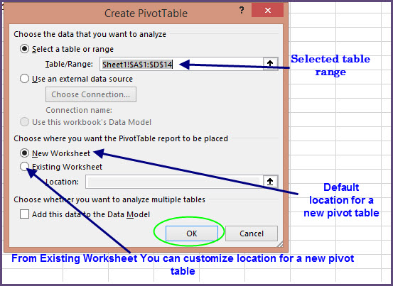
From menu bar Select Insert tab -> click on PivotTable. This will open Create Pivot Table dialog window.

    

Excel will automatically select the data for you. New Worksheet is the default location for a new pivot table. See your selected data range and default location is shown in Image.

Step 3: 

Click Ok in Create Pivot Table dialog window.
Step 4: 

Go to the new worksheet where pivot table created. 

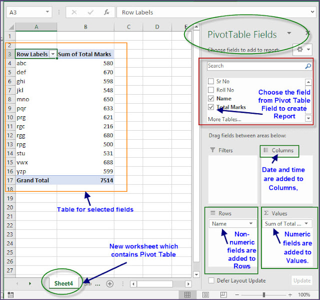
    Here You have to choose the field from Pivot Table Field to create Report as shown in Image below.
Here you can see the pivot table with your selected fields. We have selected Name and Total Marks field. Selected fields are added to their default areas, non-numeric fields are added to Rows, date and time are added to Columns, and numeric fields are added to Values.

How to Change summary Calculation in excel pivot table ?

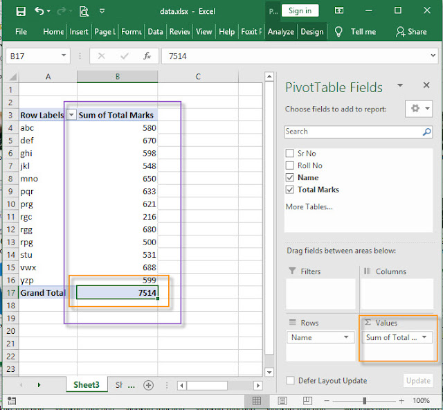
    By Default excel summarize data by summing or counting. Let’s see how to change the type of calculation?
    In Image You can see sum of total marks from data.

    Now if you want the maximum out of total marks field just follow :
Step 1:
    In Pivot Table Field Window, got to Value section and click on sum of total marks.
Step 2:
    And select Value Field Settings from pop up menu box. 

Step 3:
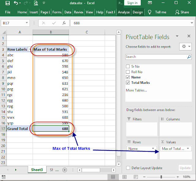
From “Value Field Settings” Select the type of calculation you want to use to summarize data from the selected field. For example, click MAX and Click OK.

Result is 688 Max of total marks will be return. Shown in Image.

I hope, you have clear Idea about Pivot table in excel. Enjoy learning.