- In today's article, we'll delve into some of the most frequently asked Excel interview questions and provide you with detailed answers to help you ace your interview. Whether you're a beginner eager to learn MS Excel or a seasoned professional looking to enhance your skills in 2024, this guide has something valuable for everyone. Let's get started!
Table of Contents
- Merging Columns with CONCATENATE and TextJoin
- Splitting Full Names into First and Last Names
- Freezing Rows for Easy Data Navigation
- Protecting Worksheets from Unwanted Changes
- Handling VLOOKUP Errors with Absolute References
- Finding the Sum of Scores with SUMIF
- Highlighting Values with Conditional Formatting
- Using Wildcards in Excel Functions
- Handling Hash Ref Errors
- Making Informed Decisions with Pivot Tables
- Preparing for Excel-Related Interviews
Merging Columns with Concatenate and TextJoin
Q: I have 3 columns called ‘First Name’, ‘Last Name’, and ‘Profession’ name. How do I merge these 3 and create a new column called, ‘full name’?
Answer:
You can achieve this by using functions like CONCATENATE and TEXTJOIN.
CONCATENATE simply combines values without a delimiter, while TEXTJOIN allows you to specify a delimiter, making it more versatile.
CONCATENATE Example in MS Excel:
In Microsoft Excel, the CONCATENATE function is used to combine multiple text strings from different cells into a single cell. This function helps you create a unified text string by joining the contents of specified cells.
Here's the syntax of the CONCATENATE function:
=CONCATENATE(text1, [text2], ...)
text1: The first text or cell reference you want to concatenate.
[text2], ...: Additional text or cell references you want to concatenate (you can include up to 255 items).
Example: CONCATENATE function
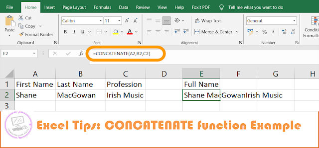
Suppose you have the following data in cells A1, B1, and C1:
A1: "Shane "
B1: "MacGowan"
C1: "Irish Music!"
You can use the CONCATENATE function to combine these strings into a single cell. In an empty cell, enter the following formula:
=CONCATENATE(A1, B1, C1)
The result will be:
Shane MacGowanIrish Music!
This formula concatenates the contents of cells A1, B1, and C1, creating a new text string that combines "Shane ," "MacGowan " (comma and space), and "Irish Music!"
TEXTJOIN Example in MS Excel Tips:
The TEXTJOIN function in Excel is used to concatenate text from multiple ranges or strings using a specified delimiter.
Example:
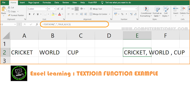
Suppose you have data in cells A1, B1, and C1 as follows:
A1: "Cricket"
B1: "World"
C1: "Cup"
You want to concatenate these strings with a comma and space as the delimiter. You can use the TEXTJOIN function with the following formula:
=TEXTJOIN(", ", TRUE, A1:C1)
Explanation of TEXTJOIN :
, : This is the delimiter that will be placed between each concatenated text.
TRUE: This argument indicates that empty cells should be ignored. If set to FALSE, empty cells would also be included in the concatenation.
A1:C1: These are the cells or ranges containing the text you want to concatenate.
The result will be:
Cricket, World, Cup
So, the TEXTJOIN function combines the text in cells A1, B1, and C1, separated by a comma and space.
Note: It's worth noting that TEXTJOIN provides a cleaner and more versatile way of concatenating text compared to older methods like CONCATENATE or the & operator.
Splitting Full Names into First and Last Names
Q: Now I want to split my ‘Full Name’ column into 2 columns with ‘first’ and ‘last’ names. How do I do that?
Sometimes, you may need to split full names into first and last names. To do this, use Excel's Text to Columns feature or Using Formulas. Ensure you clarify details with the interviewer, such as whether there may be middle names.
Splitting Text String Using Text to Columns:
- Select the column containing the full names.
- Go to the "Data" tab on the ribbon.
- In the "Data Tools" group, click on "Text to Columns."
- In the Text to Columns Wizard, choose "Delimited" and click "Next."
- Choose the delimiter that separates the first and last names (e.g., space) and click "Next."
- Choose the destination for the split data (e.g., select two adjacent columns for 'First Name' and 'Last Name') and click "Finish."
- Now, the 'Full Name' column should be split into 'First Name' and 'Last Name' columns.
Splitting Text String Using Formulas:
If you prefer using formulas, assuming your 'Full Name' is in column A, you can use the following formulas:
- For 'First Name':
=IFERROR(LEFT(A1, SEARCH(" ", A1) - 1), A1)
This formula finds the position of the space and extracts the text to the left of it as the first name.
- For 'Last Name':
=IFERROR(MID(A1, SEARCH(" ", A1) + 1, LEN(A1)), "")
This formula finds the position of the space and extracts the text to the right of it as the last name.
Drag these formulas down for the entire column to apply them to all rows.
Freezing Rows for Easy Data Navigation
Q: If you have a large dataset, and want the header row to be visible even when you scroll down, what MS Excel feature would you use?
- When working with large datasets, keeping the header row visible while scrolling is crucial. Excel offers the "Freeze Panes" feature to achieve this. You can freeze the first row or first column for better data navigation.
Steps TO freeze the Row:
- Go to the "View" tab on the ribbon.
- In the "Window" group, click on "Freeze Panes" and select "Freeze Top Row."
Protecting Worksheets from Unwanted Changes
Q: How can you prevent someone else from modifying a worksheet?
To prevent others from modifying a worksheet, use Excel's "Protect Sheet" feature. Assign permissions and set a password to restrict editing. This is particularly useful when sharing sensitive data.
To protect Worksheet:
- Go to the "Review" Tab
- Click on "Protect Sheet"
- Enter Password
To Unprotect Worksheet:
- Go to the "Review" Tab
- Click on "Unprotect Sheet"
- Enter Password if you set one.
Handling VLOOKUP Errors with Absolute References
Q: Why am I getting a #N/A when I am using my VLOOKUP Function?
Hash Ref errors in VLOOKUP functions usually result from incorrect cell references. You can avoid this by using absolute references (e.g., $A$1) to lock cell addresses. Ensure the lookup value is in the leftmost column of your data.
When you encounter a #N/A error in a VLOOKUP function, it usually indicates that the function couldn't find a match for the lookup value in the specified range. This can happen for various reasons, such as a typo, a missing value, or a mismatch between the lookup value and the data.
- Here's an example of using VLOOKUP with absolute references and handling errors:
Suppose you have the following data in columns A and B:
A B
-------------- ---------------
Employee ID Employee Name
101 John
102 Sarah
103 Michael
Now, let's say you want to use VLOOKUP to find the name of an employee with ID 104. You might use the following formula:
=VLOOKUP(104, A:B, 2, FALSE)
In this formula:
104 is the lookup value.
A:B is the table array.
2 is the column index number (Employee Name is in the second column).
FALSE is used for an exact match.
If there's no employee with ID 104, this formula will result in a #N/A error.
- To handle this error, you can use the IFERROR function along with absolute references to display a custom message or value instead. For example:
=IFERROR(VLOOKUP(104, A:B, 2, FALSE), "Employee not found")
In this formula, if the VLOOKUP results in an error, it will display the custom message "Employee not found" instead of the #N/A error.
By using absolute references and the IFERROR function, you can make your spreadsheet more user-friendly and informative when dealing with VLOOKUP errors.
Finding the Sum of Scores with SUMIF
Q: In my dataset, I have 3 columns. Student name, subject and their scores. How do I find the sum of all the scores of a single student?
Answer:
To find the sum of scores that meet specific criteria, employ the SUMIF function. Specify the range, criteria, and the range to sum. This function is valuable for data analysis.
Example of SUMIF function:
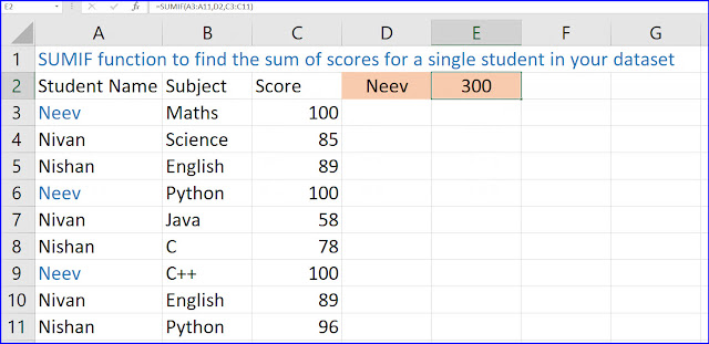
- Column A contains student names,
- Column B contains subjects, and
- Column C contains scores.
Let's say you want to find the sum of scores for the student named "Neev."
Now Enter the Student Name:
- In a new cell, enter the name of the student for whom you want to find the sum (e.g., enter "Neev" in cell E1).
Use the SUMIF Function:
In an adjacent cell (let's say cell F1), use the SUMIF function to find the sum of scores. Enter the following formula:
=SUMIF(A:A, E1, C:C)
This formula sums the scores in column C where the corresponding student name in column A matches the student name in cell E1.
A:A: This is the range of student names.
E1: This is the criteria (student name) for which you want to find the sum.
C:C: This is the range of scores.
Press Enter to calculate the sum.
Highlighting Values with Conditional Formatting
Q: From this data, how do I highlight the scores that are greater than 80?
Answer:
Conditional formatting allows you to highlight cells meeting specific conditions. For example, you can highlight scores greater than 80. Customizing cell colors enhances data visualization.
Example Step By Step to highlight value in excel sheet:
Assuming your dataset is in columns A, B, and C, where:
- Column A contains student names,
- Column B contains subjects, and
- Column C contains scores.
Select the Scores Column:
-- Click on the first cell in the "Scores" column (let's say it's C2).
-- Go to the "Home" Tab:
-- Navigate to the "Home" tab on the Excel ribbon.
-- Click on "Conditional Formatting":
-- In the "Styles" group, click on "Conditional Formatting."
-- Choose "Highlight Cells Rules" > "Greater Than":
-- From the dropdown menu, choose "Highlight Cells Rules," and then select "Greater Than."
-- Enter the Threshold (80): In the dialog box that appears, enter the value "80" as the threshold.
-- Choose Formatting Style: Choose the formatting style you want to apply to the cells with scores greater than 80. For example, you can select a fill color.
- Click "OK" to apply the formatting.
Using Wildcards in Excel Functions
Q: I have a list of subjects like History, Chemistry, Maths, Science etc. And the collective marks students have stored in each of these subjects. How do I find the total sum of scores of all the subjects ending with ‘y’?
Answer:
Wildcards like asterisks (*) and question marks (?) serve as placeholders for characters in Excel.
Use the SUMIFS function:
=SUMIFS(B:B, A:A, "*y")
Explanation:
B:B: This is the range containing the scores.
A:A: This is the range containing the subjects.
"*y": The asterisk (*) acts as a wildcard, matching any sequence of characters, and "y" specifies that the subject should end with 'y'.
The result will be the total sum of scores for subjects ending with 'y'. In this case, it would be the sum of scores for History, Chemistry, and Biology.
Handling Hash Ref Errors
Q: I deleted something and now my excel is filled with #REF errors. How do I prevent this from happening?
Hash Ref errors often occur when a formula references missing or deleted cells. Use the "Trace Dependents" feature to given in Formula tab, to identify dependent cells and avoid deleting them unintentionally.
Making Informed Decisions with Pivot Tables
Q: If I have a huge dataset of Digital Marketing spend of a company. How can I make decisions for the next marketing campaign using this data?
Pivot tables are powerful tools for analyzing and summarizing data. They allow you to pivot data for better insights, aiding decision-making in areas such as marketing budget allocation.
To excel in your Excel-related interview, ensure you're well-versed in these topics. Review Excel's capabilities in data analysis, charting, and data manipulation. Practice using functions and formulas, and explore Excel's features like conditional formatting, data validation, and more. Excel interviews can be challenging, but with proper preparation, you can confidently tackle common questions and showcase your Excel expertise.
Find Your Next Favorite Read Here
| 10 Best Excel formula to save your time
| How to use the VLOOKUP excel function ? - Easy Example
| Learn Excel Pivot Table to skill up - Simplest Example
| The best 36 Excel shortcuts to save time
| Here is different Ways of How to Divide in Excel ( with Examples )
| How to Create Drop Down List in excel, It's very very Easy
You may like to read: Run C Program on android with termux
Termux is an Android terminal emulator. The answer to the question " How to create and run C program in Android device? " Is here. To run C programs in android using Termux requires the installation of two termux packages.


0 Comments